Analytical examples

This tutorial illustrates how to define u,v velocities from two analytical fields:

1. field from a saddle point

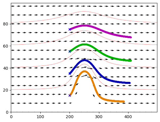
2. field around a peninsula (see in testFields.py for u,v computation)

Both example also show various particle initialization (see ParticleSet.ipynb for more details)

Import librairies

from lamta.Diagnostics import ParticleSet
import numpy as np
import matplotlib.pyplot as plt

Define saddle field

def saddle(self,t,x,y):
    Lambda=1.1
    Mu=-2.0
    xp=Lambda*x
    yp=Mu*y
    return xp,yp

Set two particles at positions px,py and time pt from user input

pt = np.array([0,1]) #time is expressed in days
numd = pt[1]- pt[0] #number of days for the integration
px = np.array([1,-1])
py = np.array([3,3])
pset = ParticleSet.from_input(pt,px,py,numdays=numd) #if numdays is not defined: default is 1
print(pset.pt,pset.px,pset.py)

[0 1] [ 1 -1] [3 3]

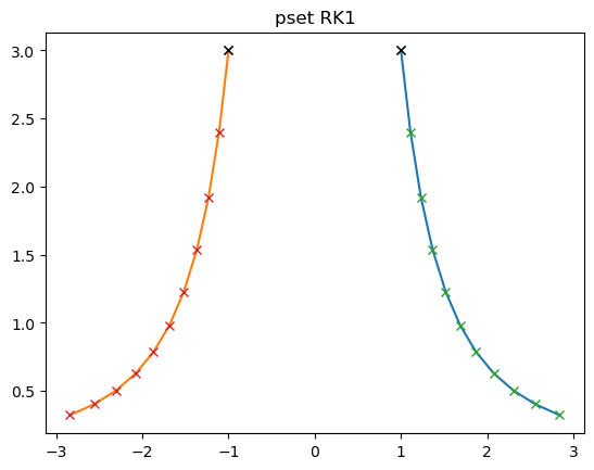
Trajectories advected with Runga-Kutta 1 with saddle field and time step=10

numstep = 10
trjf = pset.rk1flat(saddle,numstep)
print(trjf) #lons,lats = initial x,y positions; trjx,trjy = trajectories; lonf,latf = final x,y positions

{'lons': array([ 1, -1]), 'lats': array([3, 3]), 'trjx': [array([ 1, -1]), array([ 1.11, -1.11]), array([ 1.2321, -1.2321]), array([ 1.367631, -1.367631]), array([ 1.51807041, -1.51807041]), array([ 1.68505816, -1.68505816]), array([ 1.87041455, -1.87041455]), array([ 2.07616015, -2.07616015]), array([ 2.30453777, -2.30453777]), array([ 2.55803692, -2.55803692]), array([ 2.83942099, -2.83942099])], 'trjy': [array([3, 3]), array([2.4, 2.4]), array([1.92, 1.92]), array([1.536, 1.536]), array([1.2288, 1.2288]), array([0.98304, 0.98304]), array([0.786432, 0.786432]), array([0.6291456, 0.6291456]), array([0.50331648, 0.50331648]), array([0.40265318, 0.40265318]), array([0.32212255, 0.32212255])], 'lonf': [array([ 2.83942099, -2.83942099])], 'latf': [array([0.32212255, 0.32212255])]}

Plot trajectories

plt.figure()
plt.plot(trjf['trjx'],trjf['trjy'])
plt.plot(trjf['trjx'],trjf['trjy'],'x')
plt.plot(trjf['trjx'][0],trjf['trjy'][0],'kx') #plot init
plt.title('pset RK1')
plt.show()

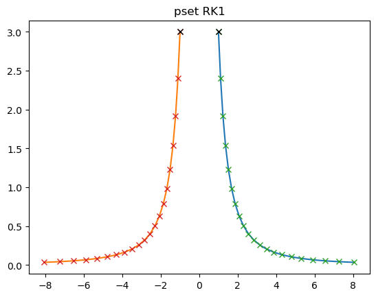
Extend to 2 days of advection

pt = np.array([0,2]) #time is expressed in days
numd = 2 #number of days for the integration
pset = ParticleSet.from_input(pt,px,py,numdays=numd) #if numdays is not defined: default is 1
numstep = 10
trjf = pset.rk1flat(saddle,numstep)
#Plot trajectories
plt.figure()
plt.plot(trjf['trjx'],trjf['trjy'])
plt.plot(trjf['trjx'],trjf['trjy'],'x')
plt.plot(trjf['trjx'][0],trjf['trjy'][0],'kx') #plot init
plt.title('pset RK1')
plt.show()

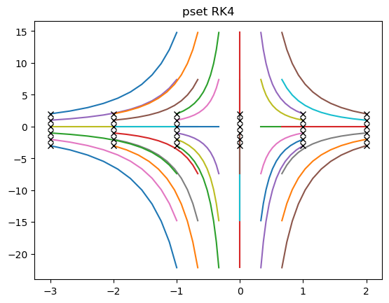
Initiate more particle (see ParticleSet.ipynb)

numdays = 1
loni = [-3,3]
lati = [-3,3]
delta0 = 1
dayv = None
pset = ParticleSet.from_grid(numdays,loni,lati,delta0,dayv)

Trajectories advected with RK4

trjf = pset.rk4flat(saddle,numstep)
print(trjf['lonf'],trjf['latf']) #show final positions

[array([-0.99861472, -0.66574315, -0.33287157,  0.        ,  0.33287157,
        0.66574315, -0.99861472, -0.66574315, -0.33287157,  0.        ,
        0.33287157,  0.66574315, -0.99861472, -0.66574315, -0.33287157,
        0.        ,  0.33287157,  0.66574315, -0.99861472, -0.66574315,
       -0.33287157,  0.        ,  0.33287157,  0.66574315, -0.99861472,
       -0.66574315, -0.33287157,  0.        ,  0.33287157,  0.66574315,
       -0.99861472, -0.66574315, -0.33287157,  0.        ,  0.33287157,
        0.66574315])] [array([-22.16666772, -22.16666772, -22.16666772, -22.16666772,
       -22.16666772, -22.16666772, -14.77777848, -14.77777848,
       -14.77777848, -14.77777848, -14.77777848, -14.77777848,
        -7.38888924,  -7.38888924,  -7.38888924,  -7.38888924,
        -7.38888924,  -7.38888924,   0.        ,   0.        ,
         0.        ,   0.        ,   0.        ,   0.        ,
         7.38888924,   7.38888924,   7.38888924,   7.38888924,
         7.38888924,   7.38888924,  14.77777848,  14.77777848,
        14.77777848,  14.77777848,  14.77777848,  14.77777848])]

Plot trajectories

plt.figure()
plt.plot(trjf['trjx'],trjf['trjy'])
plt.plot(trjf['trjx'][0],trjf['trjy'][0],'kx') #plot ini
plt.title('pset RK4')
plt.show()

Peninsula example

from testFields import peninsula
from lamta.Diagnostics import Lagrangian,ParticleSet
import numpy as np
import matplotlib.pyplot as plt

#load u,v field around peninsula
field = peninsula()

# Particle intialization from user input
pt = np.array([0,200])
px = np.array([200,200,200,200])
py = np.array([15,35,55,75])
numd = 200
pset = ParticleSet.from_input(pt,px,py,fieldset=field,numdays=numd,xy='xy') #u,v field is given as argument to be saved in pset object
#print(pset.u,pset.v) #show u,v field
#print(pset.lon)

c:\Users\lloyd\Desktop\lagrangian_dev\LAMTA_examples\notebooks\testFields.py:22: RuntimeWarning: invalid value encountered in scalar divide
  psi[i,j] = (u0*R**2*y[j]/((x[i]-x0)**2 + y[j]**2)) - u0*y[j]
C:\Users\lloyd\Desktop\lagrangian_dev\LAMTA\lamta\Diagnostics.py:1182: UserWarning: Warning: x and y data are not lon/lat
  warnings.warn("Warning: x and y data are not lon/lat")

Trajectories using RK4 method

numstep = 4
trjf = pset.rk4flat(Lagrangian.interpf,numstep)
x,y = np.asarray(trjf['trjx']),np.asarray(trjf['trjy'])

Plot field and trajectories

col = [[0.9,0.5,0],[0,0,0.7],[0,0.7,0],[0.7,0,0.7]]
plt.figure()
plt.contour(field['lon'],field['lat'],field['psi'],levels=np.arange(-80,0,20),colors='red',linewidths=0.5)
plt.quiver(field['lon'][0:500:20,0:100:8],field['lat'][0:500:20,0:100:8],field['u'][0:500:20,0:100:8],
           field['v'][0:500:20,0:100:8],scale=40)
for i in range(4):
    plt.plot(x[:,i],y[:,i],color=col[i])
    plt.plot(x[:,i],y[:,i],'.',color=col[i])
plt.plot(trjf['trjx'][0],trjf['trjy'][0],'bx')
plt.show()