Lagrangian diagnostics computation#
This notebook provides a tutorial to compute Lagrangian diagnostics from velocity fields, including:
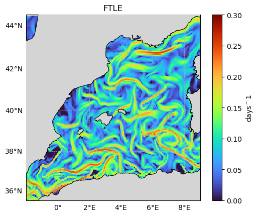
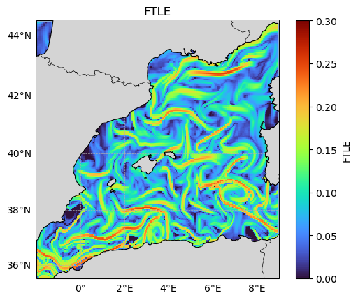
Finite-Time Lyapunov Exponents (FTLE)
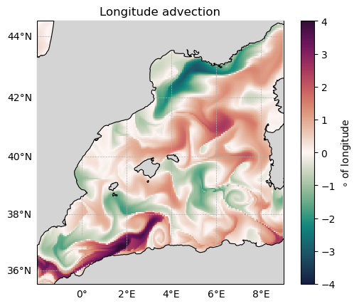
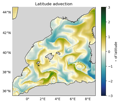
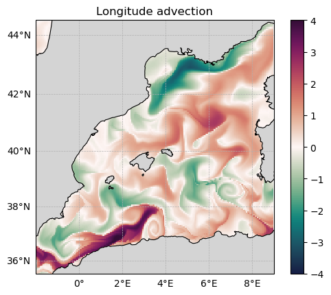
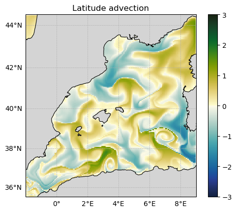
Longitude/Latitude advection (LLADV)
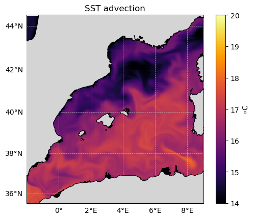
Sea Surface Temperature advection (SSTADV)
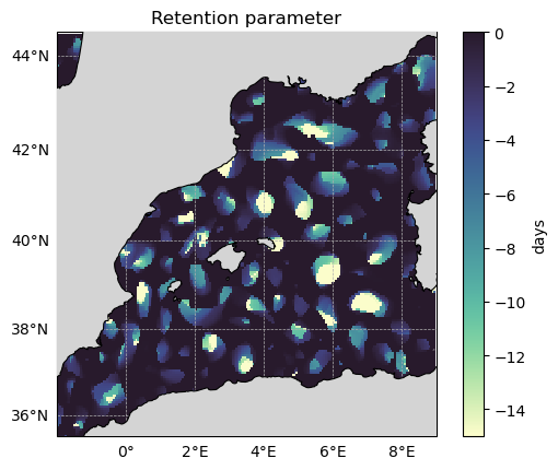
Retention parameter (OWTRAJ)
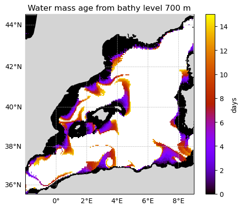
Lithogenic water mass age and transit (TIMEFROMBATHY)
The Diagnostics.Lagrangian class contains the core methods to:
Advect particles (time integration schemes, interpolation methods)
Loop over one or several diagnostics (
diag)Compute the diagnostics listed above
Diagnostics.Lagrangian first computes Lagrangian trajectories once, and then derives all requested diagnostics from these trajectories.
How to run#
Particles should first be defined using the child class ParticleSet
(see ParticleSet.ipynb).
The ParticleSet object — which contains velocity fields and particle parameters —
is then used to compute Lagrangian trajectories and derived diagnostics:
pset = Diagnostics.ParticleSet.from_XXX(args, **kwargs)
out = pset.diag(diag=[...], args, **kwargs)
Lagrangian diagnostics setup#
Lagrangian diagnostics are usually computed with particles seeded over a
regular grid in order to produce spatial maps
(using ParticleSet.from_grid()).
However, users are free to use other particle samplings.
Inputs#
Inputs for
ParticleSetare defined inParticleSet.ipynbdiag: list of diagnostics to be computedmethod: iterative method
(must have the same nomenclature as defined inDiagnostics.py)f: interpolation method
(Lagrangian.XXXinDiagnostics.py)numstep: step for the iterative methodcoordinates:"spherical"if working on Earth coordinatesnumdays: number of days for particle advectiondayv: first day of advection ("%Y-%m-%d")
Outputs#
out: array containing all diagnostics and associated variables
Example structure:
out[0]: first diagnosticout[0]['lon'],out[0]['lat'],out[0]['var0']
out[1]: second diagnostic (if applicable)out[1]['lon'],out[1]['lat'],out[1]['var1']
Note
This notebook is rendered on Read the Docs using precomputed outputs. To rerun the analysis, execute the notebook locally.
Import libraries#
from lamta.Diagnostics import ParticleSet, Lagrangian
from lamta.Save import Create
from lamta.Load_nc import loadCMEMSuv,loadsst, loadbathy
import matplotlib.pyplot as plt
import numpy as np
import cmocean as cm_oc

import cartopy.crs as ccrs
import cartopy.feature as cfeature
Fetch data#
This notebook uses reference datasets distributed via the LAMTA examples data (v0.1) GitHub release.
The data are downloaded automatically at runtime using pooch and are not stored in the repository.
Notebooks shown on Read the Docs use precomputed outputs.
To modify parameters or recompute results, run this notebook locally.
Documentation: https://lamta-examples.readthedocs.io/en/latest/
from lamta_examples.data_fetch import ensure_dataset, repo_root

DATA_DIR = ensure_dataset("altimetry_nrt_global_20220909-20220929.tar.gz")
rep = str(DATA_DIR / "altimetry" / "nrt_global") + "/"
Definition of variables#
# load field from netcdf
all_days = ['20220912','20220913','20220914','20220915','20220916','20220917','20220918','20220919','20220920','20220921','20220922','20220923','20220924','20220925','20220926','20220927','20220928','20220929']

varn = {'longitude':'longitude','latitude':'latitude','u':'ugos','v':'vgos'}
field = loadCMEMSuv(all_days,rep,varn,unit='deg/d')

# Set particles along a regular grid
numdays = 15
loni = [-2,9]
lati = [35.5,44.5]
delta0 = 0.05
dayv = '2022-09-29'
step = 10

pset = ParticleSet.from_grid(numdays,loni,lati,delta0,dayv,fieldset=field,mode='backward')
import numpy as np
import matplotlib.pyplot as plt
import cartopy.crs as ccrs
import cartopy.feature as cfeature
from cartopy.mpl.gridliner import LONGITUDE_FORMATTER, LATITUDE_FORMATTER
from matplotlib.ticker import MultipleLocator
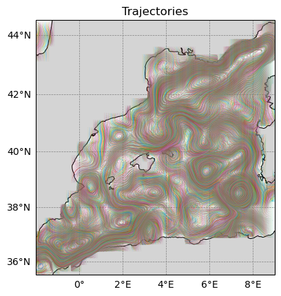
# Compute trajectories only (no diagnostics)
out = pset.diag(
diag=None,
method="rk4flat",
f=Lagrangian.interpf,
numstep=step,
coordinates="spherical",
numdays=numdays,
dayv=dayv,
)
trjf = out[0]
# Plot trajectories with Cartopy
lon_min, lon_max = loni[0], loni[1]
lat_min, lat_max = lati[0], lati[1]
fig = plt.figure()
ax = plt.axes(projection=ccrs.Mercator())
ax.set_extent([lon_min, lon_max, lat_min, lat_max], crs=ccrs.PlateCarree())
ax.add_feature(cfeature.OCEAN, facecolor="white", zorder=0)
ax.add_feature(cfeature.LAND, facecolor="0.83", edgecolor="none", zorder=1)
ax.add_feature(cfeature.COASTLINE, linewidth=0.8, zorder=2)
gl = ax.gridlines(
crs=ccrs.PlateCarree(),
draw_labels=True,
linewidth=0.5,
linestyle="--",
color="0.5",
)
gl.top_labels = False
gl.right_labels = False
gl.xformatter = LONGITUDE_FORMATTER
gl.yformatter = LATITUDE_FORMATTER
gl.xlocator = MultipleLocator(2)
gl.ylocator = MultipleLocator(2)
x = np.asarray(trjf["trjx"])
y = np.asarray(trjf["trjy"])
# Ensure shape is (ntime, ntraj)
if x.ndim == 2 and y.ndim == 2:
if x.shape[0] < x.shape[1]:
xt, yt = x, y
else:
xt, yt = x.T, y.T
else:
raise ValueError("Expected 2D trajectories arrays for trjx/trjy.")
# Break lines at NaNs (no spurious connections)
mask = np.isfinite(xt) & np.isfinite(yt)
xt = np.where(mask, xt, np.nan)
yt = np.where(mask, yt, np.nan)
ax.plot(
xt, yt,
transform=ccrs.PlateCarree(),
linewidth=0.4,
alpha=0.25,
)
ax.set_title("Trajectories")
plt.show()
import numpy as np
import matplotlib.pyplot as plt

import cartopy.crs as ccrs
import cartopy.feature as cfeature
from cartopy.mpl.gridliner import LONGITUDE_FORMATTER, LATITUDE_FORMATTER

# Compute FTLE from previous trajectories (no trajectory recomputation)
domain = ParticleSet(loni=loni, lati=lati)  # define domain only
ftle = domain.FTLE(trjf, numdays=numdays, dayv=dayv)

# Prepare grid
X, Y = np.meshgrid(ftle["lons"], ftle["lats"])  # lon/lat grid
Z = np.asarray(ftle["ftle"])                   # FTLE values

# Plot FTLE with Cartopy
fig = plt.figure()
ax = plt.axes(projection=ccrs.Mercator())

ax.set_extent([loni[0], loni[1], lati[0], lati[1]], crs=ccrs.PlateCarree())

ax.add_feature(cfeature.OCEAN, zorder=0)
ax.add_feature(cfeature.LAND, facecolor="0.83", zorder=3)
ax.add_feature(cfeature.COASTLINE, linewidth=0.8, zorder=4)
ax.add_feature(cfeature.BORDERS, linewidth=0.5, zorder=4)

pcm = ax.pcolormesh(
    X, Y, Z,
    transform=ccrs.PlateCarree(),
    cmap="turbo",
    vmin=0, vmax=0.3,
    zorder=1,
    shading="auto",
)

gl = ax.gridlines(
    crs=ccrs.PlateCarree(),
    draw_labels=True,
    linewidth=0.5,
    linestyle="--",
    zorder=5,
)
gl.top_labels = False
gl.right_labels = False
gl.xformatter = LONGITUDE_FORMATTER
gl.yformatter = LATITUDE_FORMATTER
gl.xlocator = plt.MultipleLocator(2)
gl.ylocator = plt.MultipleLocator(2)

plt.colorbar(pcm, ax=ax, label="FTLE")
ax.set_title("FTLE")
plt.show()
import numpy as np
import matplotlib.pyplot as plt

import cartopy.crs as ccrs
import cartopy.feature as cfeature
from cartopy.mpl.gridliner import LONGITUDE_FORMATTER, LATITUDE_FORMATTER

# Compute Lon/Lat advection from previous trajectories
lladv = domain.LLADV(trjf, numdays=numdays, dayv=dayv)

# plot longitude advection (LLADV)
fig = plt.figure()
ax = plt.axes(projection=ccrs.Mercator())

ax.set_extent([loni[0], loni[1], lati[0], lati[1]], crs=ccrs.PlateCarree())

X, Y = np.meshgrid(lladv["lons"], lladv["lats"])

pcm = ax.pcolormesh(
    X, Y, lladv["lonf_map"],
    transform=ccrs.PlateCarree(),
    cmap=cm_oc.cm.curl,
    vmin=-4, vmax=4,
    shading="auto",
    zorder=1,
)

ax.add_feature(cfeature.LAND, facecolor="0.83", zorder=2)
ax.add_feature(cfeature.COASTLINE, linewidth=0.8, zorder=3)

gl = ax.gridlines(
    crs=ccrs.PlateCarree(),
    draw_labels=True,
    linewidth=0.5,
    linestyle="--",
)
gl.top_labels = False
gl.right_labels = False
gl.xformatter = LONGITUDE_FORMATTER
gl.yformatter = LATITUDE_FORMATTER
gl.xlocator = plt.MultipleLocator(2)
gl.ylocator = plt.MultipleLocator(2)

plt.colorbar(pcm, ax=ax)
ax.set_title("Longitude advection")
plt.show()

# plot latitude advection (LLADV)
fig = plt.figure()
ax = plt.axes(projection=ccrs.Mercator())

ax.set_extent([loni[0], loni[1], lati[0], lati[1]], crs=ccrs.PlateCarree())

X, Y = np.meshgrid(lladv["lons"], lladv["lats"])

pcm = ax.pcolormesh(
    X, Y, lladv["latf_map"],
    transform=ccrs.PlateCarree(),
    cmap=cm_oc.cm.delta,
    vmin=-3, vmax=3,
    shading="auto",
    zorder=1,
)

ax.add_feature(cfeature.LAND, facecolor="0.83", zorder=2)
ax.add_feature(cfeature.COASTLINE, linewidth=0.8, zorder=3)

gl = ax.gridlines(
    crs=ccrs.PlateCarree(),
    draw_labels=True,
    linewidth=0.5,
    linestyle="--",
)
gl.top_labels = False
gl.right_labels = False
gl.xformatter = LONGITUDE_FORMATTER
gl.yformatter = LATITUDE_FORMATTER
gl.xlocator = plt.MultipleLocator(2)
gl.ylocator = plt.MultipleLocator(2)

plt.colorbar(pcm, ax=ax)
ax.set_title("Latitude advection")
plt.show()
from pathlib import Path

outdir = Path("..") / "outputs"
outdir.mkdir(parents=True, exist_ok=True)

# Save previous outputs in netcdf files
fname = outdir / "FTLE_test.nc"
title = "FTLE 2022-09-29"
var_name = "ftle"
var_units = "d^{-1}"
Create.netcdf(str(fname), ftle["lons"], ftle["lats"], ftle["ftle"], title, var_name, var_units)

Create.netcdf(
    str(outdir / "LLADV_test.nc"),
    lladv["lons"], lladv["lats"], lladv["lonf_map"],
    "LLADV 2022-09-29", "lonf_map", "degreeE",
    var2=lladv["latf_map"], var2_name="latf_map", var2_units="degreeN",
)
Compute trajectories and all diagnostics at once#
# 1) Ensure the SST dataset bundle is present
DATA_DIR = ensure_dataset("sst_ostia_slstr_samples.tar.gz")

# 2) Point rep to the OSTIA folder
rep_sst = str(DATA_DIR / "sst" / "ostia") + "/"

# 3) Load SST
sstname = "20230109120000-UKMO-L4_GHRSST-SSTfnd-OSTIA-GLOB-v02.0-fv02.0.nc"
sstfield = loadsst(sstname, rep_sst)

# additional parameters
bathylvl = -700 # in meters

# Ensure bathymetry bundle is available
DATA_DIR = ensure_dataset("bathymetry_etopo_medsea.tar.gz")

# Point to the correct subfolder
rep_bathy = str(DATA_DIR / "bathymetry") + "/"

# Load bathymetry
bathyname = "ETOPO_2022_v1_30s_N90W180_bed_MedSea.nc"
bfield = loadbathy(
    bathyname,
    rep_bathy,
    rlon=loni,
    rlat=lati,
)

# Lagrangian diagnostics computation
out = pset.diag(diag=['LLADV','FTLE','OWTRAJ','SSTADV','TIMEFROMBATHY'],method='rk4flat',
                f=Lagrangian.interpf,numstep=step,
                coordinates='spherical',numdays=numdays,dayv=dayv,
                ds=1/6,sstfield=sstfield,bathyfield=bfield,
                bathylvl=bathylvl)

trjf = out[0]
lladv = out[1]
ftle = out[2]
owdisp = out[3]
sstadv = out[4]
timfb = out[5]
C:\Users\lloyd\Desktop\lagrangian_dev\LAMTA\lamta\Diagnostics.py:494: UserWarning: Warning: 'daysst' is not defined -> using default value (3)
  warnings.warn("Warning: 'daysst' is not defined -> using default value (3)")
import numpy as np
import matplotlib.pyplot as plt
import cartopy.crs as ccrs
import cartopy.feature as cfeature
from cartopy.mpl.gridliner import LONGITUDE_FORMATTER, LATITUDE_FORMATTER
def _cartopy_base_ax(loni, lati):
"""Create a Cartopy Mercator axes with the same extent and labelled gridlines."""
fig = plt.figure()
ax = plt.axes(projection=ccrs.Mercator())
ax.set_extent([loni[0], loni[1], lati[0], lati[1]], crs=ccrs.PlateCarree())
gl = ax.gridlines(
crs=ccrs.PlateCarree(),
draw_labels=True,
linewidth=0.5,
linestyle="--",
)
gl.top_labels = False
gl.right_labels = False
gl.xformatter = LONGITUDE_FORMATTER
gl.yformatter = LATITUDE_FORMATTER
gl.xlocator = plt.MultipleLocator(2)
gl.ylocator = plt.MultipleLocator(2)
return fig, ax
def _cartopy_pcolormesh(ax, lons, lats, field, **kwargs):
"""pcolormesh in lon/lat coords (PlateCarree) onto a projected axes."""
X, Y = np.meshgrid(lons, lats)
return ax.pcolormesh(
X, Y, field,
transform=ccrs.PlateCarree(),
shading="auto",
**kwargs,
)
def _add_continents_on_top(ax, facecolor="0.83"):
"""Add land/coastlines above data (continents on top)."""
# Land on top of the raster
ax.add_feature(cfeature.LAND, facecolor=facecolor, zorder=100)
ax.add_feature(cfeature.COASTLINE, linewidth=0.8, zorder=101)
# plot FTLE
fig, ax = _cartopy_base_ax(loni, lati)
pcm = _cartopy_pcolormesh(
ax, ftle["lons"], ftle["lats"], ftle["ftle"],
cmap="turbo", zorder=-1, vmin=0, vmax=0.3,
)
_add_continents_on_top(ax, facecolor="0.83")
cbar = plt.colorbar(pcm, ax=ax)
cbar.set_label("days$^-{1}$")
plt.title("FTLE")
plt.show()
# plot LLADV
fig, ax = _cartopy_base_ax(loni, lati)
pcm = _cartopy_pcolormesh(
ax, lladv["lons"], lladv["lats"], lladv["lonf_map"],
cmap=cm_oc.cm.curl, zorder=-1, vmin=-4, vmax=4,
)
_add_continents_on_top(ax, facecolor="0.83")
cbar = plt.colorbar(pcm, ax=ax)
cbar.set_label("$\\circ$ of longitude")
plt.title("Longitude advection")
plt.show()
fig, ax = _cartopy_base_ax(loni, lati)
pcm = _cartopy_pcolormesh(
ax, lladv["lons"], lladv["lats"], lladv["latf_map"],
cmap=cm_oc.cm.delta, zorder=-1, vmin=-3, vmax=3,
)
_add_continents_on_top(ax, facecolor="0.83")
cbar = plt.colorbar(pcm, ax=ax)
cbar.set_label("$\\circ$ of latitude")
plt.title("Latitude advection")
plt.show()
# plot Retention parameter
fig, ax = _cartopy_base_ax(loni, lati)
pcm = _cartopy_pcolormesh(
ax, owdisp["lons"], owdisp["lats"], owdisp["owdisp"],
cmap=cm_oc.cm.deep, zorder=-1, vmin=-15, vmax=0,
)
_add_continents_on_top(ax, facecolor="0.83")
cbar = plt.colorbar(pcm, ax=ax)
cbar.set_label("days")
plt.title("Retention parameter")
plt.show()
# plot SST advection
fig, ax = _cartopy_base_ax(loni, lati)
pcm = _cartopy_pcolormesh(
ax, sstadv["lons"], sstadv["lats"], sstadv["sstadv"],
cmap="inferno", zorder=-1, vmin=14, vmax=20,
)
_add_continents_on_top(ax, facecolor="0.83")
cbar = plt.colorbar(pcm, ax=ax)
cbar.set_label("$\\circ$C")
plt.title("SST advection")
plt.show()
# plot time from bathy (water mass age)
fig, ax = _cartopy_base_ax(loni, lati)
pcm = _cartopy_pcolormesh(
ax, timfb["lons"], timfb["lats"], timfb["timfb"],
cmap="gnuplot", zorder=-1, vmin=0, vmax=15,
)
_add_continents_on_top(ax, facecolor="0.83")
cbar = plt.colorbar(pcm, ax=ax)
cbar.set_label("days")
plt.title("Water mass age from bathy level 700 m")
plt.show()
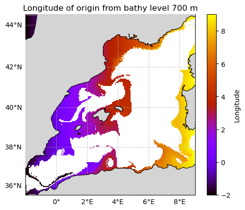
# plot longitude from bathy (transit)
fig, ax = _cartopy_base_ax(loni, lati)
pcm = _cartopy_pcolormesh(
ax, timfb["lons"], timfb["lats"], timfb["lonfb"],
cmap="gnuplot", zorder=-1, vmin=-2, vmax=9,
)
_add_continents_on_top(ax, facecolor="0.83")
cbar = plt.colorbar(pcm, ax=ax)
cbar.set_label("Longitude")
plt.title("Longitude of origin from bathy level 700 m")
plt.show()
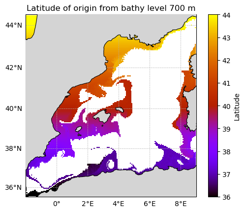
# plot latitude from bathy (transit)
fig, ax = _cartopy_base_ax(loni, lati)
pcm = _cartopy_pcolormesh(
ax, timfb["lons"], timfb["lats"], timfb["latfb"],
cmap="gnuplot", zorder=-1, vmin=36, vmax=44,
)
_add_continents_on_top(ax, facecolor="0.83")
cbar = plt.colorbar(pcm, ax=ax)
cbar.set_label("Latitude")
plt.title("Latitude of origin from bathy level 700 m")
plt.show()